5. Probing and Finetuning

5.1 Manually Downloading Data

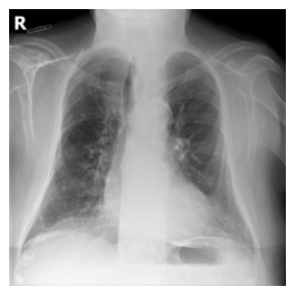
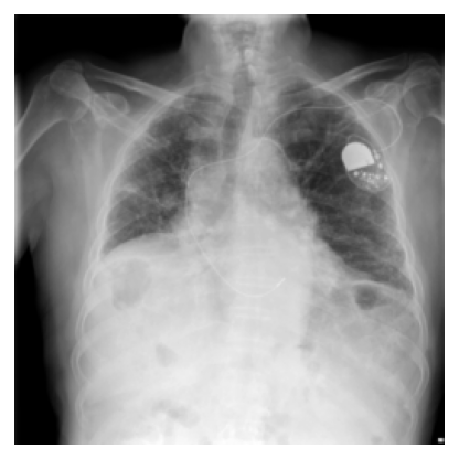
The evaluation dataset is PadChest (160,000 chest X-rays from Hospital Universitario de San Juan with 174 radiographic finding labels annotated by NLP from radiology reports). It is fully public, you just fill out a form, get approved, get access.

One thing I've noticed about this project is how much it relies on open science infrastructure. The NIH dataset is public. PadChest is public. The fact that I could run this entire project on a $0 budget is not an accident.

The PadChest download was not, however, a simple wget.

After approval, the data comes as numbered zip files, each around 20GB. I needed enough labeled examples of each rare disease to run a meaningful evaluation, roughly 20–50 per class after the train/val split. The problem is that any given zip contains maybe 3 examples of a rare finding. To accumulate enough, I had to download about 18 of these zips over the course of a week, totaling roughly 350GB.

I couldn't automate it. The download endpoint required manually click onto each file. So I would queue one up, wait 1-2 hours, find out it had disconnected due to bad connection, restart it, finally download it, then start the next one. After filtering to frontal projections (PA and AP), I ended up with approximately 34,500 usable images.

5.2 Choosing Which Diseases to Evaluate

I excluded common diseases with large public labeled datasets: pneumonia, pleural effusion, cardiomegaly, atelectasis, nodule, emphysema. These are what NIH ChestX-ray14 and CheXpert were built to cover, not self-supervised learning.

I excluded non-specific radiological descriptors: "increased density," "infiltrates," "chronic changes," "bronchovascular markings." These are descriptions of what the image looks like, not disease entities.

I excluded structural and age-related variants: vertebral degenerative changes, kyphosis, aortic elongation, azygos lobe. These are normal anatomical variants that appear with age, not diseases.

Clarification: I excluded "rib fracture" but kept "callus rib fracture." A callus rib fracture is a healing fracture showing new bone formation, a specific radiological sign with no large public labeled dataset. The generic "rib fracture" is excluded because NIH has rib fracture annotations; callus rib fracture stays because it doesn't.

Only single-label images are used. A multi-label image is ambiguous for binary classification as the model can't learn a clean signal for any single finding. Around half of usable AP/PA images are multi-labelled and subsequently discarded.

excluded: 5 labels

pulmonary fibrosis, chronic changes, kyphosis, pseudonodule, ground glass pattern

included: 1 label

pulmonary fibrosis

Further nuance: train/val split is done at the patient level, not the image level. PadChest contains follow-up scans so the same patient may have multiple X-rays taken over several years. If you split by image, those scans scatter across train and val, and the model learns patient-specific anatomy rather than disease features.

The fix is to have all images from a patient go to either train or val, never both. The assignment uses a hash of the patient ID, making it reproducible regardless of download order. This is also why the split is an approximate 80/20 rather than precisely 80/20.

import hashlib

# each CSV row looks like:
# ImageID:    185923405191181100399370637716198851619_9l64ns.png
# PatientID:  123706734192256204891233254155489787944
# Projection: PA
# Labels:     ['bronchiectasis']

# by_patient maps each PatientID to all their single-label PA/AP scans:
# { "123706734...": [(Path("zip_0/img.png"), "bronchiectasis"), ...], ... }
by_patient: dict[str, list[tuple[Path, str]]] = {}
for row in csv.DictReader(f):
    patient_id = row["PatientID"].strip()
    by_patient.setdefault(patient_id, []).append((path, label))

# Hash-stable split: reproducible regardless of zip ordering.
val_patients = {
    pid
    for pid in by_patient
    if int(hashlib.md5(pid.encode()).hexdigest(), 16) % round(1 / val_frac) == 0
}

train_by_label: dict[str, list[Path]] = {}
val_by_label: dict[str, list[Path]] = {}
for patient_id, samples in by_patient.items():
    target = val_by_label if patient_id in val_patients else train_by_label
    for path, label in samples:
        target.setdefault(label, []).append(path)

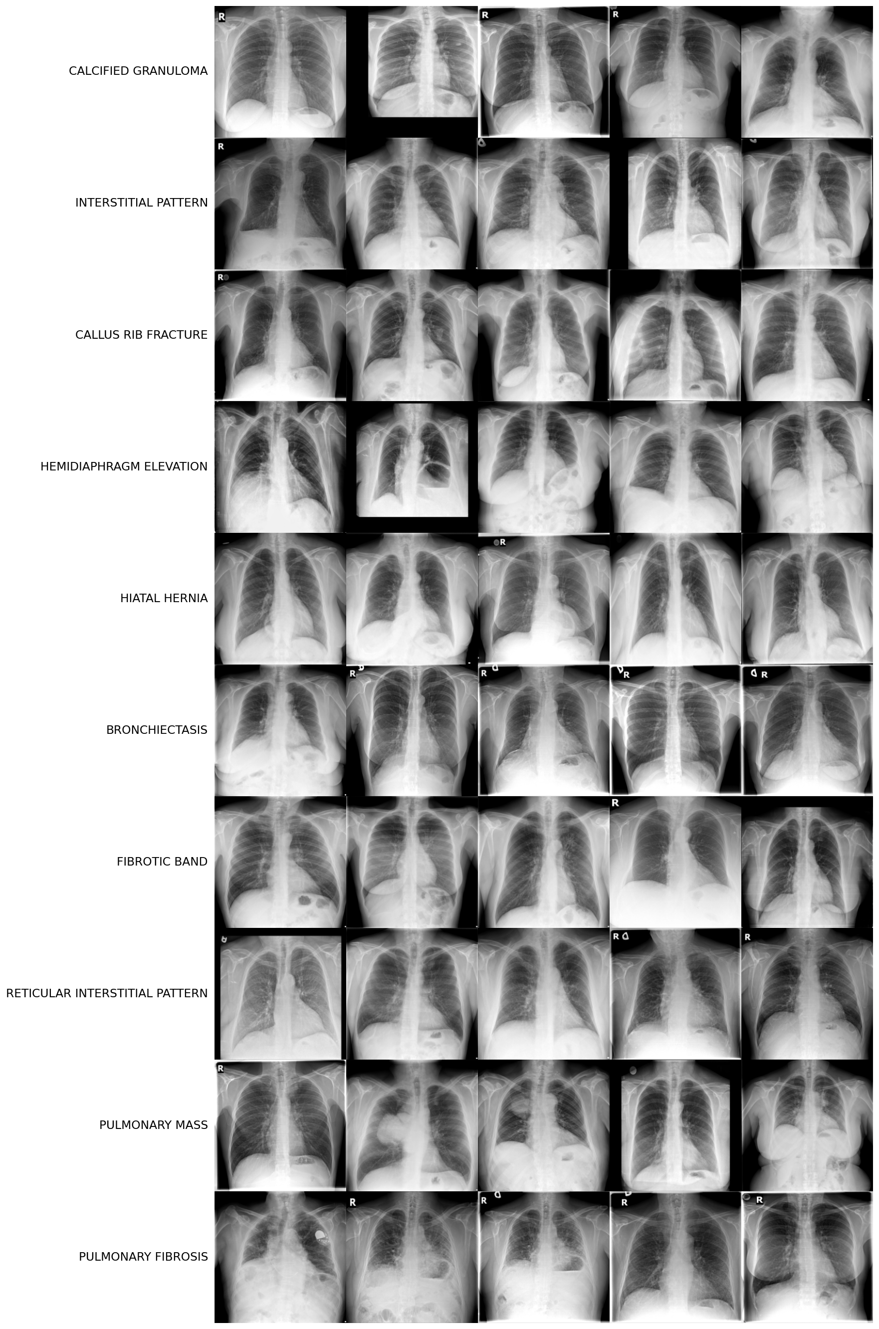
After applying all filters and setting the count threshold to a minimum 15 train examples and 4 val examples, 10 disease classes remained:

5.3 Domain Gap Analysis: NIH to PadChest

In Part 1, I described how COVID classifiers hit 95–98% "accuracy" while actually detecting hospital-specific marker fonts and other spurious data. Pretraining on NIH and evaluating on PadChest was a direct defense against that repeating. If self-supervised learning memorized NIH-specific artifacts (scanner exposure profiles, black border padding, English annotation overlays), those shortcuts won't survive a transfer to PadChest.

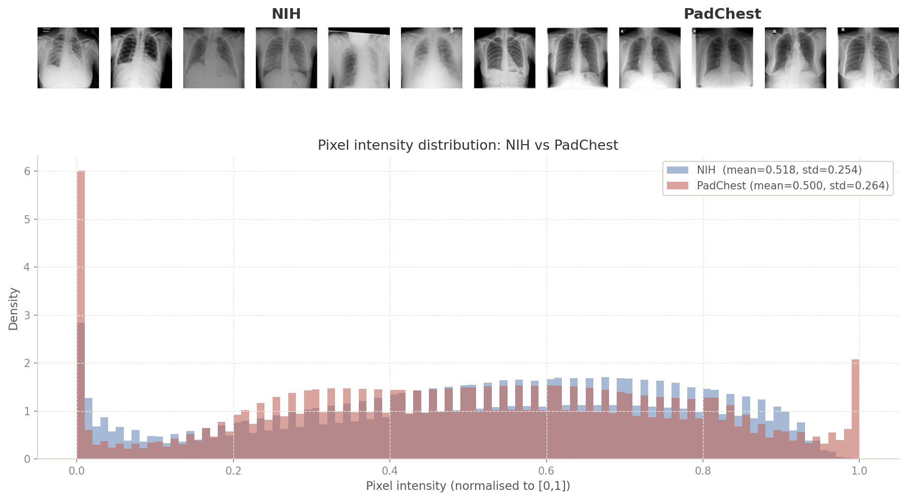
I was curious whether there even was a scanner gap to worry about (even if there was, it would be made redundant by our pretraining augmentations). I measured pixel-level statistics (mean intensity and standard deviation) across a random sample of images from each dataset to find out.

from PIL import Image

def _load_gray(path: Path) -> np.ndarray:
    img = Image.open(path).convert("L").resize((224, 224))
    return np.array(img, dtype=np.float32) / 255.0

# flatten all pixels from 500 sampled images into one array
rng = random.Random(42)
nih_pixels = np.concatenate([_load_gray(p).ravel() for p in rng.sample(nih_paths, 500)])
pc_pixels = np.concatenate([_load_gray(p).ravel() for p in rng.sample(padchest_paths, 500)])

mean_shift = abs(nih_pixels.mean() - pc_pixels.mean())
std_ratio = nih_pixels.std() / pc_pixels.std()

# NIH: mean=0.518, std=0.254
# PadChest: mean=0.500, std=0.264
# mean_shift=0.018
# std_ratio=0.961

A mean shift of 0.018 is negligible. NIH and PadChest frontal X-rays are essentially identically distributed at the pixel level.

5.4 Probing vs Finetuning: What's the Difference?

For each disease at each shot count, I run two evaluations: a linear probe and a gradient finetune. Here is how they differ.

Linear probe: The backbone is completely frozen. Features are extracted once, and a logistic regression head is fit on those frozen features. No gradient updates touch the backbone. It measures what the backbone actually learned with no chance of compensating for bad features.

Finetuning: Gradient updates flow through unfrozen backbone layers plus a linear head. The backbone adapts to the downstream task. The linear head is initialized using prototypical initialization where the weight vector for each class is set to the L2-normalized mean of that class's support features. This gives the head a reasonable starting point without wasting our already limited training data on finding the class separation.

Finetuning is what you'd actually deploy, but with very few labeled examples it can also overfit on the backbone weights. I wanted to see which one of these methods would produce better results.

5.5 Surgically Unfreezing: Why These Layers?

Before deciding which layers to freeze, I built and ran a GradCAM (Gradient-weighted Class Activation Mapping) at each ResNet stage to see exactly what spatial information each layer was encoding. It backpropagates the classifier score through the target layer, global-average-pools the gradients to get per-channel importance weights, weights the forward activations by those, and applies ReLU. The result is a heatmap over the input showing where that layer "looked."

# gradients flow back through the target layer via a backward hook
weights = self.gradients.mean(dim=(2, 3), keepdim=True)
cam = F.relu((weights * self.activations).sum(dim=1, keepdim=True))
cam = F.interpolate(cam, size=(224, 224), mode="bilinear")

Attaching GradCAM to each ResNet layer in sequence shows a clear progression:

• Layer1: responds to high-contrast edges across the entire X-ray: ribs, cardiac borders, lung margins equally.
• Layer2: starts to cluster but is still broad.
• Layer3: activations begin localizing to the lower chest and diaphragm region where a hiatal hernia sits.
• Layer4: tight focal hotspot at exactly that location.

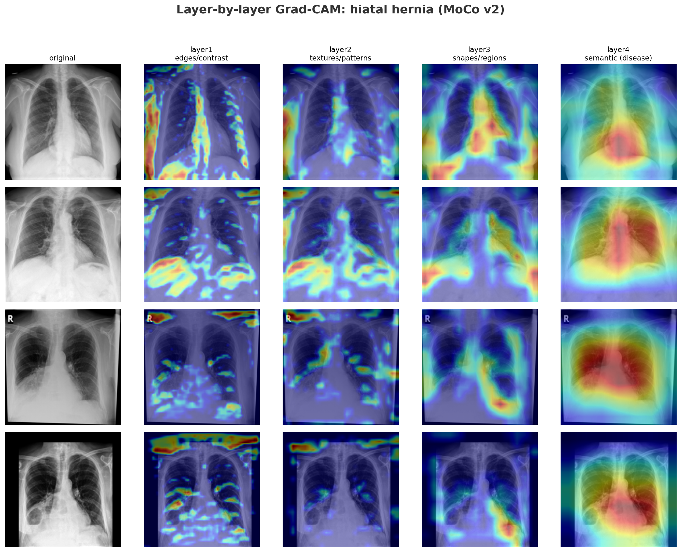
MoCo's layer2 encodes chest-specific structural context: rib cage geometry, lung field boundaries, and mediastinal shape, which serves as the scaffolding layers 3 and 4 build upon to localize disease. Because MoCo's layer2 is calibrated by a global contrastive loss at layer4 learning which cues pull similar whole images together, unfreezing layer2+ allows the model to reweight those structural features specifically for the target disease.

SparK's layer2 also encodes chest anatomy, but through a different supervision. Instead of a global objective, it receives pixel-level gradients directly from the decoder's skip connection optimizing it to represent spatial anatomy patch by patch.

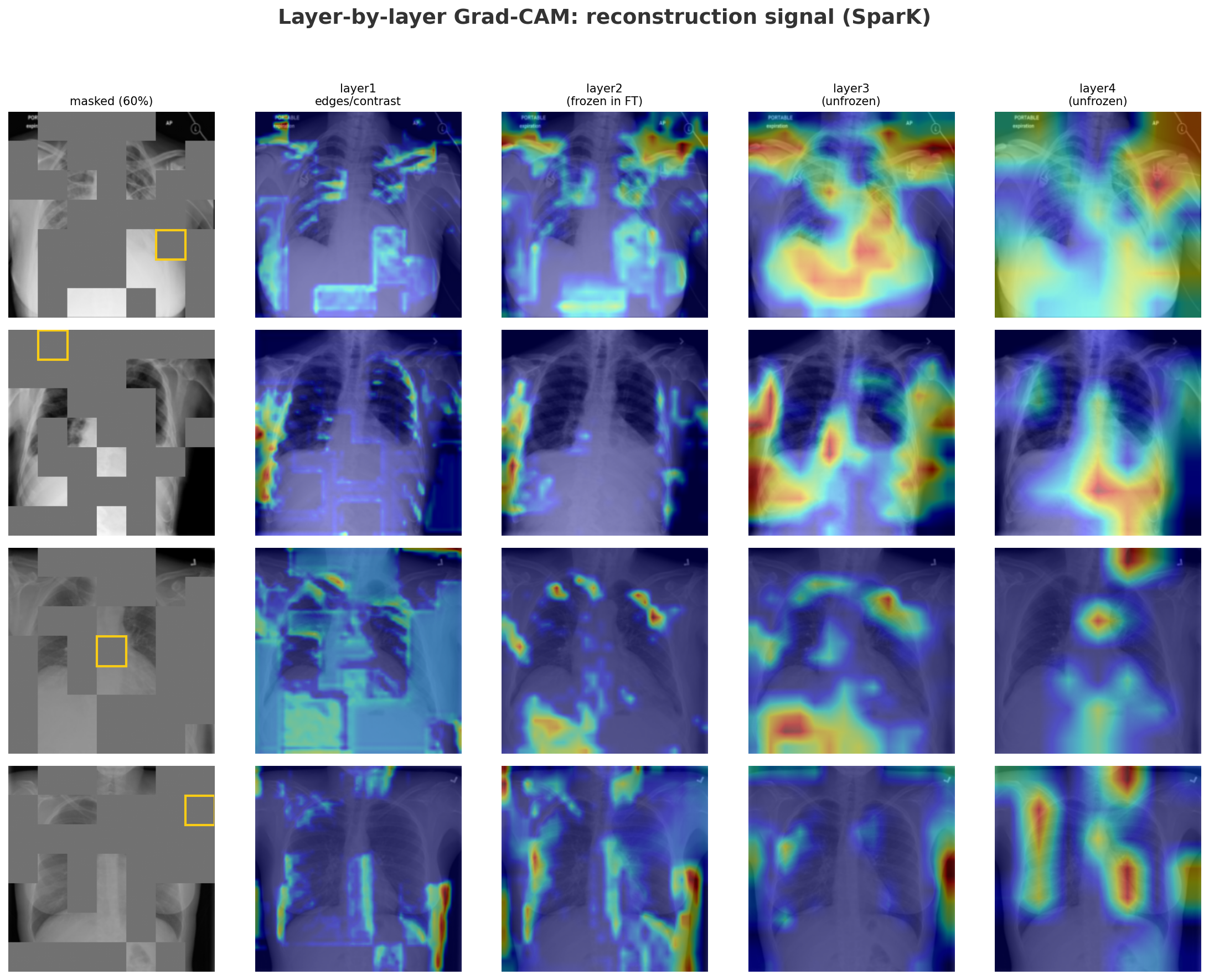
The reconstruction GradCAM shows that even for a single missing patch (yellow box), layer2 already draws on the right structural context, with layer3 and layer4 progressively narrowing in. Finetuning on only a handful of labeled examples means there is nothing to gain by adjusting layer2 further without a bigger risk of overfitting. That's why we unfreeze layer3+ for SparK.

Finally, we always keep BatchNorm frozen: the batch normalization statistics were computed over 112,000 NIH images during pretraining. Unfreezing Batch Normalization on just a few dozen examples would cause it to overfit on that tiny sample and destabilize training.

5.6 N-shot Protocol and Training Setup

I finetuned across a sweep of 1, 5, 10, 20, and 50 "shots", where "shot" refers to the number of labeled examples per class provided to the downstream task. As mentioned in Motivation, the upside of SSL is its ability to produce useful representations even in extreme low-data regimes like 1-shot (where the model sees exactly one labeled X-ray per disease). This sweep lets us test how quickly performance improves as labeled data accumulates and compare it to other baselines.

Class balance: Each n-shot training set samples exactly N positive and N negative examples. Without this, a model minimizing cross-entropy on rare diseases would just default to predicting everything as "no disease". However, the validation set still retains its imbalanced distribution just like in a real world medical setting, which is why we use AUC as our evaluation metric rather than accuracy.

Learning rates: The backbone and head are optimized with a differential learning rate: lr_backbone=1e-4 and lr_head=1e-3. The backbone updates ten times slower to preserve the pretrained features; the head can move faster because prototype initialization already gives it the right class geometry. Both decay to zero over 100 epochs via cosine annealing.