Part 3 of 6 in the SCARCE-CXR series
3.1 SSL Archetypes
SSL methods are categorized into three families.
- Contrastive methods (SimCLR, MoCo, BarlowTwins) learn by comparison. Push representations of two augmented views of the same image together, and push representations of different images apart. The signal comes from the relationships between examples.
- Self-distillation methods (BYOL, SimSiam, DINO) drop explicit negative pairs entirely. A student network is trained to match a teacher network (usually a slowly-evolving EMA copy of the student). The signal comes from the teacher's soft assignments.
- Generative methods (MAE, BEiT, SparK) learn by reconstruction. They mask a large fraction of the input and force the network to hallucinate what was hidden based on the surrounding structure. The signal comes from pixel-level and patch-level context.
3.2 MoCo v2: Lineage and Compute Constraints
I had high hopes for contrastive learning on chest X-rays because dataset homogeneity is irrelevant. The question is "did these two views come from the same image?" regardless of how similar everything else looks. Augmentation diversity matters; dataset diversity doesn't.
MoCo v1 first made contrastive learning doable on a single GPU by storing negatives (embeddings from other images, used as contrast) in a 65,536-entry queue. SimCLR then dropped the queue, proving you could just use other images in the same batch as negatives. It worked elegantly, but there was one problem: it required a massive batch size of 4096 across 32 TPUs we didn't have, and passing 4096 augmented pairs through a ResNet50 wouldn't come close to fitting in my single L4 GPU's 22GB of VRAM. We needed a way to graft SimCLR's representation improvements back onto MoCo's queue-based architecture.
MoCo v2 was selected because it has the architectural answers to our compute bottleneck.
3.3 MoCo v2: Model Internals
MoCo's loss function is called InfoNCE. Given a query
embedding q
and a key
k from two crops of the same image, pick
k out of a crowd of negatives from other images.
The positive pair is always placed at position 0 in the logits,
so cross-entropy does the rest. If the embeddings collapse
and everything looks the same, the positive wins by default
and loss drops for the wrong reason.
# q and k are L2-normalized embeddings from two crops of the same image
l_pos = torch.einsum("nc,nc->n", q, k).unsqueeze(-1) # (N, 1): how similar is q to its match?
l_neg = torch.einsum("nc,ck->nk", q, queue) # (N, 65536): similarity against every negative in the queue

# InfoNCE: disguise SSL as a 65,537-way classification problem
logits = torch.cat([l_pos, l_neg], dim=1) / T # glue into one lineup; T sharpens the distribution
labels = torch.zeros(N, dtype=torch.long) # correct answer is always index 0
loss = F.cross_entropy(logits, labels)
MoCo v2 refined this further: the authors grafted SimCLR's MLP projection head and stronger augmentations onto the original queue design, and got similar results without a TPU cluster. On one L4 GPU with 22GB of VRAM, it was exactly the right architecture for this dataset.
Beyond the queue, MoCo v2 has two more structural defenses against collapse:
1. Momentum encoder: a slowly-evolving shadow copy of the query encoder, updated by EMA rather than gradient descent, so the keys in the queue stay consistent. If the key encoder updated as fast as the query encoder, old queue entries would become stale and the negatives meaningless.
2. MLP projection head: the contrastive loss can distort the backbone's feature space in arbitrary ways to satisfy its objective. The projection head absorbs those distortions, leaving the backbone representations clean. After pretraining, the head is thrown away.
On paper, there's no easy path to a degenerate solution.
# From ssl_methods/moco/model.py

# 1. Momentum encoder (EMA): slowly-evolving shadow copy, updated without gradients
@torch.no_grad()
def _momentum_update(self):
    for p_q, p_k in zip(self.encoder_q.parameters(), self.encoder_k.parameters()):
        p_k.data = p_k.data * self.m + p_q.data * (1.0 - self.m) # m=0.999: key encoder moves 0.1% per step

# 2. MLP projection head: swap ResNet's fc classifier for a 2-layer bottleneck
def build_encoder(encoder_name: str, dim: int):
    backbone = getattr(models, encoder_name)(weights=None)
    feature_dim = backbone.fc.in_features
    backbone.fc = nn.Sequential(
        nn.Linear(feature_dim, feature_dim), # first layer: 2048 -> 2048
        nn.ReLU(),
        nn.Linear(feature_dim, dim), # second layer: 2048 -> 128
    )
    return backbone

# called in __init__:
self.encoder_q = build_encoder(encoder_name, dim) # query encoder: updated by gradient descent
self.encoder_k = build_encoder(encoder_name, dim) # key encoder: separate instance, then weights copied below
for p_q, p_k in zip(self.encoder_q.parameters(), self.encoder_k.parameters()):
    p_k.data.copy_(p_q.data) # start identical to encoder_q
    p_k.requires_grad = False # no gradients ever; EMA updates only

# forward pass: where #1 and #2 meet the InfoNCE loss
q_raw = self.encoder_q(x_q) # raw 128-d output before normalization; VICReg variance term fires on these
q = F.normalize(q_raw, dim=1) # L2-normalize so dot products become cosine similarities

with torch.no_grad():
    self._momentum_update() # k = m*k + (1-m)*q: EMA drifts encoder_k so old queue entries stay valid
    k = F.normalize(self.encoder_k(x_k), dim=1) # key: momentum encoder only, no gradients flow here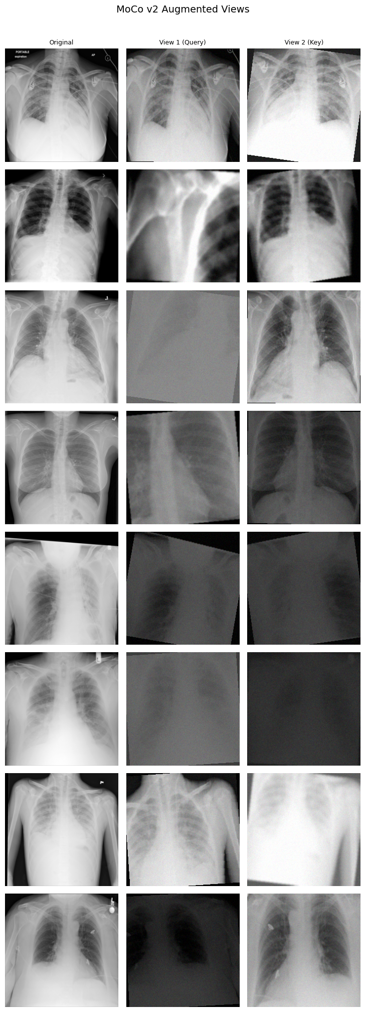
encoder_q and encoder_k.
Each row is one image; the model never sees the
original on the left.Besides, temperature T=0.07 makes the ranking task brutally hard. The model is penalized for not pushing the positive pair to the absolute top of 65,536 entries, so I started the first training run pretty confident the architecture had collapse handled.
3.4 How to Fix Feature Collapse
But of course it didn't. Around epoch 100, the training loss was dropping faster and smoother than it had any right to. That kind of smooth descent usually means the model found a shortcut: collapse to a narrow subspace, make all embeddings similar, and the InfoNCE task becomes trivially easy because the positive pair always wins by default.
So I built collapse_monitor.py to diagnose it.
Every few epochs it samples 2,048 embeddings and computes
three numbers:
# From data/eval/collapse_monitor.py
def compute_metrics(feats: np.ndarray) -> tuple[float, float, float]:
    mean_std = float(feats.std(axis=0).mean()) # near 0 = collapsed

    norms    = np.linalg.norm(feats, axis=1, keepdims=True)
    normed   = feats / (norms + 1e-8)
    rng      = np.random.default_rng(0)
    n_pairs  = min(2048, len(normed) * (len(normed) - 1) // 2)
    idx_a, idx_b = rng.integers(0, len(normed), n_pairs), rng.integers(0, len(normed), n_pairs)
    mean_cos = float((normed[idx_a] * normed[idx_b]).sum(axis=1).mean()) # near 1 = collapsed

    centered = feats - feats.mean(axis=0)
    _, sv, _ = np.linalg.svd(centered, full_matrices=False)
    sv       = sv / sv.sum()
    sv       = sv[sv > 0]
    eff_rank = float(np.exp(-(sv * np.log(sv)).sum())) # near 1 = single direction used

    return mean_std, mean_cos, eff_rank
The first run confirmed the suspicion:
| Epoch | std | mean_cos | eff_rank |
|---|---|---|---|
| 50 | 0.363 | 0.675 | 175.6 |
| 100 | 0.162 | 0.533 | 219.3 |
| 200 | 0.061 | 0.446 | 251.7 |
| 264 | 0.060 | 0.393 | 261.8 |
The std column is the thing to look at. It dropped
from 0.363 to 0.060 by epoch 264, then flatlined. The model
was squeezing everything into a narrow cone in the latent
space. InfoNCE alone, on data this homogeneous, couldn't keep
all 128 dimensions alive.
My first fix was stronger augmentations. More aggressive crops, higher jitter, Gaussian noise to simulate X-ray quantum noise. I updated the config: crop scale from [0.2, 1.0] to [0.08, 1.0], brightness and contrast jitter from 0.4 to 0.8, noise at std=0.1. Each change has a physical justification (section 2.2). But it still wasn't enough. As I later learned, stronger augmentations make the pretext task harder; they don't directly penalize dimensional collapse. On data this homogeneous, the model kept finding the lazy path.
When I looked at related SSL literature for more something structural, I found an actual fix: VICReg. It has a variance term that fires whenever any projection dimension's standard deviation drops below 1.0. I pulled just that one term and applied it directly to the unnormalized query projections:
# From ssl_methods/moco/train.py
def variance_loss(z: torch.Tensor, gamma: float = 1.0) -> torch.Tensor:
std = torch.sqrt(z.var(dim=0) + 1e-4)
return F.relu(gamma - std).mean()
infonce = F.cross_entropy(logits, labels)
var = variance_loss(q_raw) # applied to pre-normalized projections
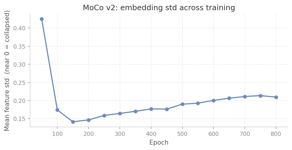
loss = infonce + 1.0 * varIt worked. On the next run (800 epochs, batch size 384), std
bottomed out at 0.142 around epoch 150 then climbed back to
0.215 by epoch 800.
mean_cos fell to 0.435 and
eff_rank stabilized near 219. VICReg caught the
collapse mid-run and reversed it.

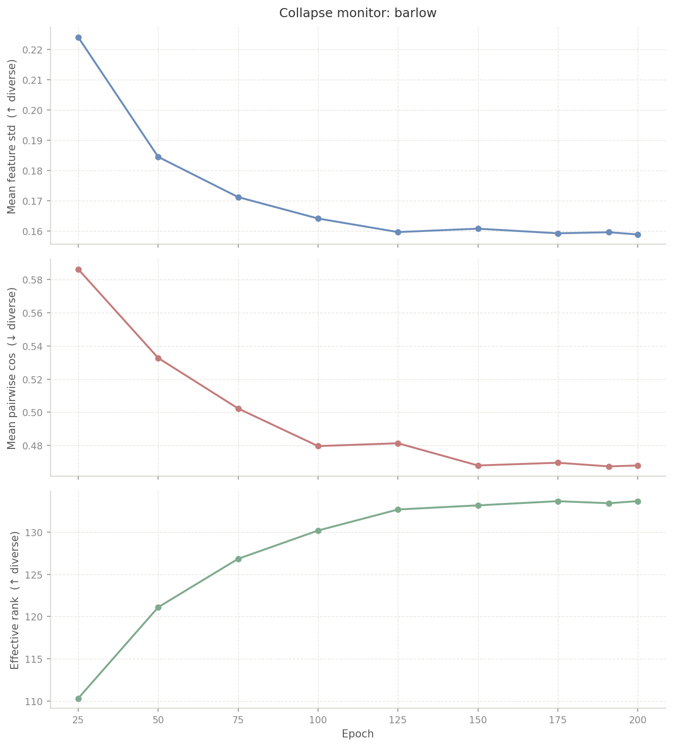
3.5 BarlowTwins: An Elegant Alternative
MoCo took 800 epochs and an intervention to get right. After all that, it was worth asking: do we actually need the queue, the momentum encoder, and the EMA update? Or can we get good representations without any of that?
BarlowTwins strips out all of that. No negative queue, no shadow encoder, no temperature tuning. Both views pass through the same backbone in the same forward pass. The only question is: do the two views produce the same embedding, and are the embedding dimensions non-redundant? The entire method lives in the loss:
# From ssl_methods/barlow/loss.py
z1 = (z1 - z1.mean(0)) / (z1.std(0) + 1e-6) # batch-normalize so C is a true correlation matrix, not a covariance
z2 = (z2 - z2.mean(0)) / (z2.std(0) + 1e-6)

# cross-correlation matrix (2048, 2048): how correlated is each dimension of z1 with each dimension of z2?
c = z1.T @ z2 / N

# pull diagonal to 1: the same image seen two ways should produce the same features
on_diag = (torch.diagonal(c) - 1).pow(2).sum()
# push off-diagonal to 0: each dimension should carry information the others don't
off_diag = _off_diagonal(c).pow(2).sum()

loss = on_diag + 0.005 * off_diag # λ=0.005: small, but there are 2048²-2048 off-diagonal entries so it adds up
_off_diagonal extracts those entries without
allocating a new matrix:
# From ssl_methods/barlow/loss.py
def _off_diagonal(x):
    n, m = x.shape
    assert n == m
    return x.flatten()[:-1].view(n-1, n+1)[:, 1:].flatten()
# flatten to 1D, drop last element to prevent row wraparound,
# reshape to (n-1, n+1), slice off column 0 (diagonal entries), flatten again
1. Diagonal term: enforces invariance: the same image, augmented two ways, should produce the same features.
2. Off-diagonal term: enforces decorrelation: if two dimensions always move together, one of them is redundant.
Together they rule out collapse without any contrastive negative pairs. The forward pass reflects the same simplicity. Compare this to MoCo's two encoders, EMA update, and queue:
# From ssl_methods/barlow/model.py (forward pass)
# one shared backbone: both views update the same weights simultaneously
z1 = self.projector(self._encode(x1)) # view 1: backbone + projector → 2048-d
z2 = self.projector(self._encode(x2)) # view 2: identical path, same weights

# gradient checkpointing: instead of storing all intermediate activations for backward,
# recompute them on demand, reduces activation memory at the cost of a second forward pass
x = ckpt.checkpoint(bb.layer1, x, use_reentrant=False)
x = ckpt.checkpoint(bb.layer2, x, use_reentrant=False) # applied across all 4 layer blocks
3.6 BarlowTwins: How to Reason About OOM
MoCo wraps encoder_k in
torch.no_grad(), so only the query encoder
builds a gradient graph. BarlowTwins has no such
shortcut: both views go through the same backbone and
both need gradients.
The first run I tried was ResNet50 at N=512. OOM. I dropped it to 384. Still OOM. Dropped to 256. OOM. Tried 320. OOM. At that point it was clear the batch size was not the problem.
So I dug into what PyTorch was actually holding in
memory. Without gradient checkpointing,
loss.backward() needs the full computation graph
intact: every intermediate activation from every conv across
both views, all in memory at the same time.
# ResNet50, no checkpointing, N=512, both views
# each layer's spatial resolution is the grid of positions the conv slides over
# 56x56 = 3,136 positions per channel; memory scales with positions x channels x batch

#                                   spatial grid  channels     activation memory
stem: downsamples input 224x224 to  56x56         64ch         ~0.6GB
layer1: 3 blocks, stays at          56x56         64->256ch    ~13.1GB  # most expensive: largest grid + widening channels
layer2: 4 blocks, halves to         28x28         256->512ch   ~13.4GB  # first block straddles both resolutions
layer3: 6 blocks, halves to         14x14         512->1024ch  ~8.3GB   # smaller grid but more channels
layer4: 3 blocks, halves to         7x7           1024->2048ch ~3.4GB   # tiny grid, cheapest layer
                                                              ---------
                                                        total: ~38.8GB

# halving the batch halves everything: at N=256 total drops to ~19.4GB.
# still over 22GB once params, gradients, and optimizer state are added.
The problem is structural. Layer1 and Layer2 dominate because they process the largest spatial grids. Each conv at 56x56 stores 3,136 values per channel per image. With 256 channels and 512 images per batch, that is over 400 million floats per tensor, and there are dozens of tensors. Cutting the batch size in half cuts memory in half, but 19.4GB at N=256 still exceeds what the L4 can hold once everything else is added.
The fix was to switch to ResNet18. The two backbones are structurally different, not just smaller. ResNet18 uses basic blocks: two 3×3 convs with a skip connection. ResNet50 uses bottleneck blocks: a 1×1 to compress channels, a 3×3 for spatial features, and a 1×1 to expand back.
flowchart LR
    x["x"] --> c1["3×3 conv\nspatial"]
    c1 --> c2["3×3 conv\nspatial"]
    c2 -->|"F(x)"| add["⊕"]
    x -->|"skip connection"| add
    add -->|"F(x) + x"| relu["ReLU"]
flowchart LR
    x["x"] --> c1["1×1 conv\nreduce channels"]
    c1 --> c2["3×3 conv\nspatial"]
    c2 --> c3["1×1 conv\nexpand channels"]
    c3 -->|"F(x)"| add["⊕"]
    x -->|"skip connection"| add
    add -->|"F(x) + x"| relu["ReLU"]
The full architectures stack these blocks across four stages. ResNet50 widens to 256 channels at layer1 while still at 56×56, and keeps widening from there. ResNet18 stays at 64 channels at layer1 and uses simpler 2-conv blocks throughout.
flowchart LR
    inp["input\n224×224"] --> stem["stem\n7×7 conv /2\nmax pool /2\n56×56×64"]
    stem --> s1["stage 1\n×2 blocks\n56×56×64"]
    s1 --> s2["stage 2\n×2 blocks\n28×28×128"]
    s2 --> s3["stage 3\n×2 blocks\n14×14×256"]
    s3 --> s4["stage 4\n×2 blocks\n7×7×512"]
    s4 --> gap["global\navg pool\n512-d"]
    gap --> out["SSL head\n(discarded)"]
flowchart LR
    inp["input\n224×224"] --> stem["stem\n7×7 conv /2\nmax pool /2\n56×56×64"]
    stem --> s1["stage 1\n×3 blocks\n56×56×256"]
    s1 --> s2["stage 2\n×4 blocks\n28×28×512"]
    s2 --> s3["stage 3\n×6 blocks\n14×14×1024"]
    s3 --> s4["stage 4\n×3 blocks\n7×7×2048"]
    s4 --> gap["global\navg pool\n2048-d"]
    gap --> out["SSL head\n(discarded)"]
ResNet18 stays at 64 channels at layer1 and never expands past 512 channels total. Fewer channels at the expensive 56×56 resolution is the key difference. On top of switching backbones, gradient checkpointing was added. Checkpointing discards every intermediate activation during the forward pass and recomputes them during backward only when needed. Only the layer boundary outputs are kept throughout:
# From ssl_methods/barlow/model.py (_encode)
def _encode(self, x):
    bb = self.backbone
    x = bb.maxpool(bb.relu(bb.bn1(bb.conv1(x)))) # stem: 224×224 → 56×56
    x = ckpt.checkpoint(bb.layer1, x, use_reentrant=False) # discard intermediates, keep output
    x = ckpt.checkpoint(bb.layer2, x, use_reentrant=False) # same for each stage
    x = ckpt.checkpoint(bb.layer3, x, use_reentrant=False)
    x = ckpt.checkpoint(bb.layer4, x, use_reentrant=False)
    return bb.avgpool(x).flatten(1) # 7×7 → 512-d
With checkpointing, the retained memory drops to just the four layer outputs, held for both views:
# ResNet18, gradient checkpointing, N=512 (layer boundary tensors only)
layer1 out: 512 × 64 × 56 × 56  = 103M floats
layer2 out: 512 × 128 × 28 × 28 = 51M floats
layer3 out: 512 × 256 × 14 × 14 = 26M floats
layer4 out: 512 × 512 × 7 × 7   = 13M floats
# activations: 193M × 2 views × 4 bytes = ~1.4GB
# optimizer (AdamW m+v, ~21M params) = ~0.2GB
# total: ~1.6GB. Fits at N=512 with room to spare.
ResNet18 with gradient checkpointing fit batch size 512
and runs roughly 4× faster per epoch. And unlike MoCo,
there was no collapse to fix. std
settled at 0.161 by epoch 125 and held there for the remaining
75 epochs. The decorrelation loss handles collapse directly
by construction.