Part 4 of 6 in the SCARCE-CXR series
4.1 DINO: Self-Distillation and Architectural Guardrails
Contrastive learning works by comparison: pull two views of the same image together, push views of different images apart. That second part needs different images in the batch to push against, which is why batch size and memory queues are so critical. Self-distillation drops the negatives entirely. A "student" network does not compare against other images at all. Instead, it learns to match the output of a "teacher" network for the exact same image.
The problem is that without negatives pushing embeddings apart, the network finds the laziest solution: output the same constant vector for every image and drive the loss to zero. Early methods like BYOL dealt with this through architectural guardrails: an asymmetric predictor head on the "student" side only, plus a stop-gradient on the "teacher". These worked empirically; remove either one and training collapses. But nobody fully understood why the asymmetry prevented collapse. We needed a mathematically transparent way to prevent collapse, not one that just "worked" somehow .
DINO replaces those tricks with a mechanism one can actually reason about: a centring buffer (more on that next). If it fails, you know exactly what to look at. On ImageNet with ViT backbones, it worked well enough to produce attention maps that trace object boundaries without any human supervision. That result convinced me it should generalize anywhere.
4.2 DINO: Model Internals
Compared to MoCo v2, the infrastructure needed drops significantly. MoCo v2 holds a 65,536-entry queue in GPU memory, large batches to keep those negatives diverse, and computes a loss that pits every query against all 65,536 stored embeddings. DINO has none of that:
| MoCo v2 | DINO | |
|---|---|---|
| Negatives | 65,536-entry queue of past embeddings | None |
| Batch-size sensitivity | High; queue needs diverse images | Low |
| Loss compares | query against all 65,536 queue entries | "teacher"/"student" crop pairs from current batch |
| Collapse prevention | negatives push embeddings apart | centring buffer + temperature asymmetry |
| Extra GPU memory | 65,536 × 128-dim queue | K-dim centring vector |
The architecture is simple. Both the "student" and "teacher" share the same structure: a backbone followed by a DINOHead projection head outputting out_dim=65,536 logits. The "teacher" never receives gradients; its weights slowly track the "student" via EMA.
# From ssl_methods/dino/model.py

# Both share the same architecture: backbone → DINOHead (3-layer MLP → L2-norm → 65536-dim linear)
self.student = nn.Sequential(backbone_s, DINOHead(feature_dim, out_dim=65536))
self.teacher = nn.Sequential(backbone_t, DINOHead(feature_dim, out_dim=65536))

# 1. EMA "teacher": weights drift toward "student" via EMA
for p in self.teacher.parameters():
    p.requires_grad = False # "teacher" never updated by gradient descent

@torch.no_grad()
def update_teacher(self, momentum: float):
    for p_s, p_t in zip(self.student.parameters(), self.teacher.parameters()):
        p_t.data = p_t.data * momentum + p_s.data * (1.0 - momentum) # at momentum=0.996, only 0.4% per step

# Forward: "student" sees all crops, "teacher" only sees global crops
student_out = [self.student(v) for v in views]
with torch.no_grad():
    teacher_out = [self.teacher(views[i]) for i in range(n_global)]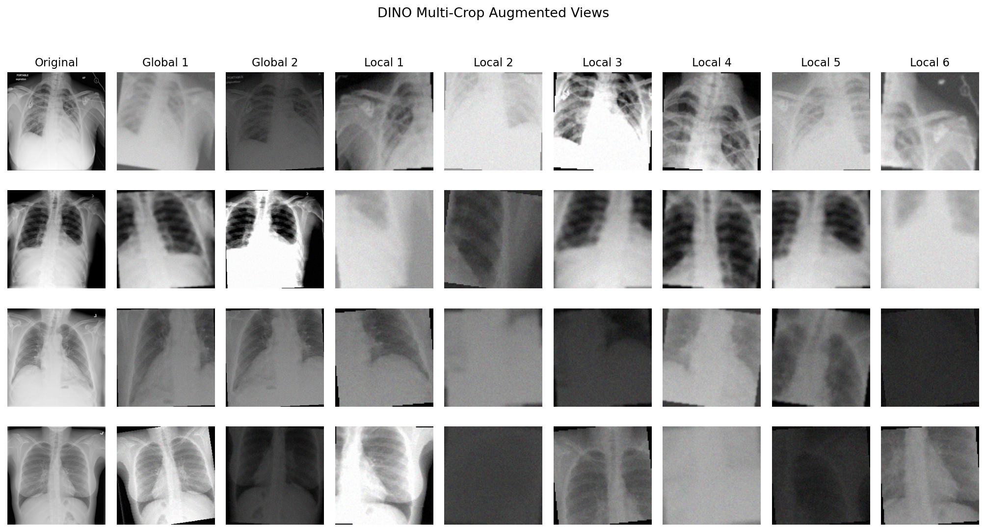
DINO's loss is a cross-entropy between two probability distributions. The "teacher" passes each global crop through a projection head to get K=65,536 logits, applies centring and a low temperature to produce a sharp, peaked distribution, then detaches from the graph. The "student" processes all crops and must match those distributions.
# From ssl_methods/dino/loss.py

# 2. Temperature asymmetry: teacher_temp=0.04
# 3. Centring buffer: subtract center
teacher_probs = [
    F.softmax((t - self.center) / self.teacher_temp, dim=-1).detach()
    for t in teacher_output # peaked distribution, no gradients
]
# 2. Temperature asymmetry: student_temp=0.1 for softer distribution
student_log_probs = [
    F.log_softmax(s / self.student_temp, dim=-1)
    for s in student_output # all crops; higher temp keeps distribution softer
]

# Cross-entropy over all (teacher_i, student_j) pairs, skip same-view
total_loss -= torch.mean(torch.sum(t_prob * s_lp, dim=-1))

# 3. Centring buffer: update running mean
batch_center = torch.cat(teacher_output).mean(dim=0, keepdim=True)
self.center = self.center * self.center_momentum + batch_center * (1.0 - self.center_momentum)
Three structural choices keep the system from collapsing:
1. EMA "teacher": the "teacher" never receives gradients. Its weights drift toward the "student" each step by exponential moving average. A fast-updating "teacher" would produce an inconsistent training signal. At momentum=0.996 it moves only 0.4% per step, providing a stable target.
2. Temperature asymmetry: teacher_temp=0.04 makes the "teacher"'s distribution sharp and peaked. student_temp=0.1 keeps the "student" softer. Matching a peaked target forces the "student" to concentrate probability mass on the same prototypes, not approximate a uniform distribution.
3. Centring buffer: a running mean is subtracted from the "teacher" logits before softmax. If all mass concentrates on one output dimension, the running mean tracks and subtracts it, flattening that bias out and preventing single-prototype collapse.
4.3 DINO: Plateauing Loss
The centring buffer assumes that different images produce meaningfully different "teacher" outputs. That assumption holds on ImageNet. It does not hold here.
On ImageNet, a dog produces a wildly different "teacher"
output than a car. But chest X-rays share the same modality,
gross anatomy, and grayscale range, so the "teacher" assigns
near-identical probability distributions to everything. The
running center average converges to the default output for
any image. Then t - self.center
approaches zero, and softmax(0 / 0.04) returns
a uniform distribution. The "student" is asked to match a
flat line. There is no gradient signal. We confirmed this by
running
collapse_monitor.py on the DINO checkpoints: mean
pairwise cosine similarity climbed steadily while effective rank
fell, both signatures of collapse.
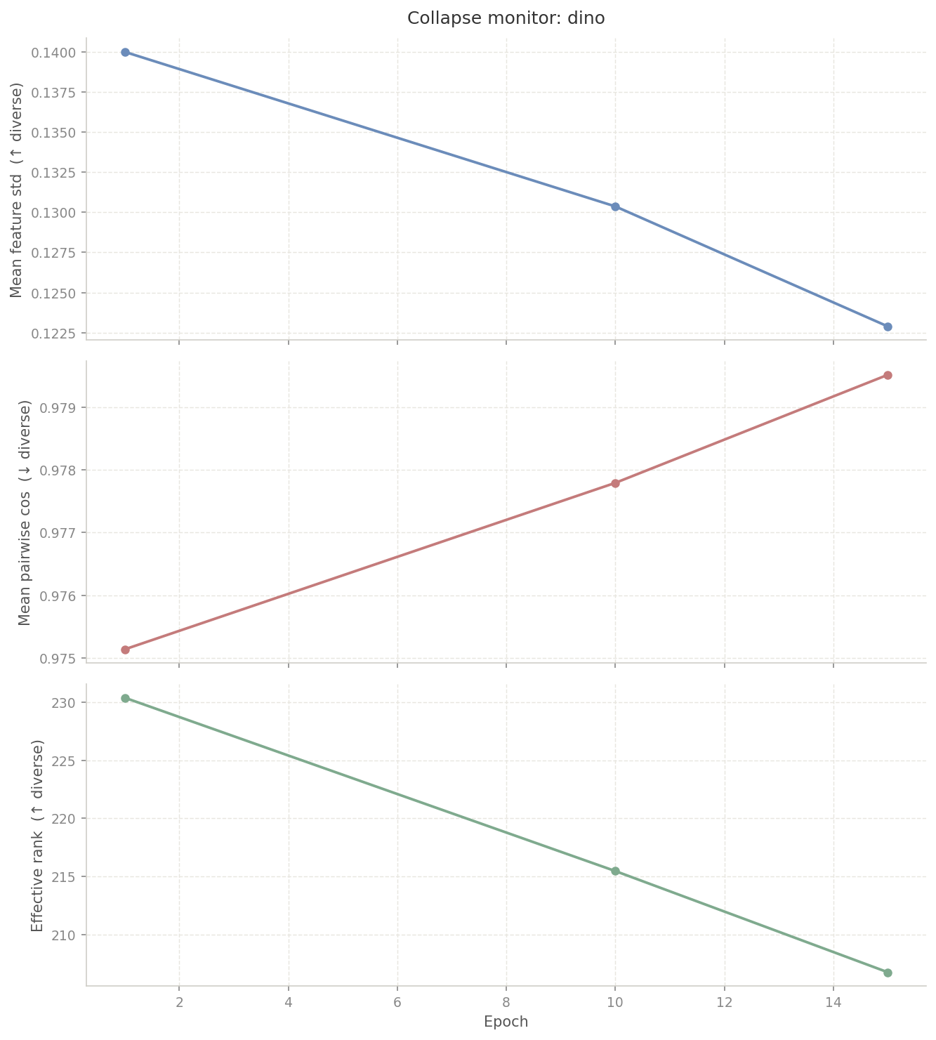
Our loss flatlined at 5.42 and never moved beyond that. I tried the standard fixes: dropping output dimension, raising centre momentum to 0.99, adjusting the "teacher" temperature warmup, disabling local crops. None of it moved the loss.

Takeaway: DINO's self-distillation requires visual diversity that chest X-rays simply do not have.
4.4 SparK: Generative Models and Convolution Leakage
Contrastive learning has a blind spot when applied to X-rays: augmentation invariance. The model is rewarded for ignoring differences between two crops of the same image, but a fibrotic band or a tiny nodule is so subtle that two crops of the same X-ray look nearly identical with or without it. Contrastive learning has little incentive to preserve a microscopic feature.
In 2018, BERT transformed NLP by masking random words in a sentence and training a model to predict them from context. That idea became the dominant pretraining recipe in language, and MAE applied the same logic to vision: mask out 75% of image patches, then reconstruct them. It worked extremely well. But ViTs treat images as sequences of discrete patch tokens so masking is clean and no information leaks across boundaries. CNNs were systematically left out of this entire line of progress. SparK changed that by basically designing BERT for convolutional networks.
flowchart LR
    bert["BERT (2018)\nNLP\n─────────────\nmask random words\npredict from context"]
    mae["MAE (2021)\nVision Transformer\n─────────────\nmask patches\nreconstruct image"]
    spark["SparK (2023)\nConvolutional Network\n─────────────\nmask pixel space\nreconstruct via U-Net"]

    bert --> mae
    mae --> spark
A ViT was not an option at our scale. They have no spatial inductive bias and need over a million images to learn useful patch relationships. Given our smaller dataset with essential spatial relations, a ViT would underfit badly. A ResNet was the only viable backbone. But simply slapping a ResNet on a MAE introduces two problems:
1. Convolutional leakage: standard convolutions slide their kernels across the image and leak visible pixel data into masked regions, allowing the model to cheat.
2. Spatial resolution loss: ResNets compress a 224x224 image down to a 7x7 grid, permanently destroying the high-frequency detail needed to reconstruct smaller features.
SparK is the architectural fix for both.
4.5 SparK: Model Internals
SparK asks the question: given some patches of an image, can the network reconstruct the rest? The whole architecture follows from that change.
The forward pass has four stages.
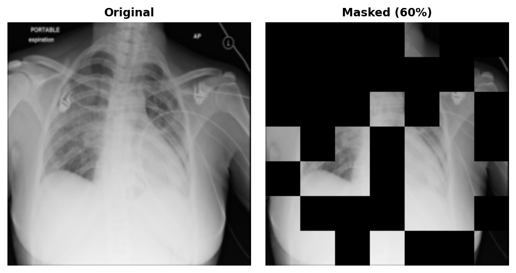
1. Masking. Before the first convolution, the 224x224 input is divided into non-overlapping 32x32 patches. 60% are randomly selected and zeroed out in raw pixel space. This is the key architectural difference from MAE: a ViT only processes tokens for visible patches, so masked content never enters the computation at all. A CNN has no such luxury: convolutional kernels slide over the entire image regardless. Masking in pixel space before the first convolution is necessary, but it does not prevent leakage on its own. The paper's solution is sparse convolutions that physically skip masked positions entirely.
2. Encoding. The masked image passes through the standard ResNet50 stem and four residual stages, producing hierarchical feature maps at progressively coarser spatial resolutions: f1 at 56x56, f2 at 28x28, f3 at 14x14, and f4 at 7x7 (the bottleneck).
3. Decoding. A lightweight U-Net decoder upsamples from the 7x7 bottleneck back to 224x224 using skip connections from f1, f2, and f3. Without those skips, the decoder would have to hallucinate sharp ribs and vasculature from a 7x7 grid (geometrically impossible).
flowchart TB
    inp["input 224x224 (masked)"]
    inp --> f1["f1: 56x56, 256ch"]
    f1  --> f2["f2: 28x28, 512ch"]
    f2  --> f3["f3: 14x14, 1024ch"]
    f3  --> f4["f4: 7x7, 2048ch (bottleneck)"]
    f4  --> d3["upsample to 14x14 + f3 skip"]
    d3  --> d2["upsample to 28x28 + f2 skip"]
    d2  --> d1["upsample to 56x56 + f1 skip"]
    d1  --> out["reconstruction 224x224"]
    f3 -.->|skip| d3
    f2 -.->|skip| d2
    f1 -.->|skip| d1
4. Loss. The target is the original unmasked image, with each 32x32 patch normalised to zero mean and unit variance before computing the loss. MSE is evaluated on masked pixels only:
# From ssl_methods/spark/model.py

# Normalise each 32x32 patch to zero mean, unit variance
# Guessing the average grey value now yields 0 on mean but still fails on variance
# To minimise MSE, the network must reconstruct the actual high-frequency edges
target = self._patchwise_normalize(x)

# MSE on masked regions only (same idea as BERT: loss only on [MASK] tokens)
# visible pixels are in the input; including them lets the decoder copy for free
loss = ((pred - target) ** 2 * mask_px).sum() / (mask_px.sum() * x.shape[1])
4.6 SparK: When Blind Implementations Don't Work
Deploying the original theory within our compute constraints (a single 22GB GPU) required three specific implementation fixes.
Fix 1: Input-level masking instead of per-stage sparse simulation. The original SparK simulates sparse convolution using standard PyTorch operators: after each residual stage, it re-applies a downsampled version of the mask to the feature map, zeroing masked positions before the next stage sees them. This prevents masked-region values from accumulating across layers. This implementation takes the simpler route: zero masked patches once at input and run standard Conv2d through all four stages. The leakage cost is real but bounded, and on 112k images rather than ImageNet's 1.28M the easier pretext task is the right call.
# From ssl_methods/spark/model.py

def _random_mask(self, imgs):
    B, C, H, W = imgs.shape
    p = self.patch_size # 32
    nh, nw = H // p, W // p # 7×7 = 49 patches total
    n_mask = int(nh * nw * self.mask_ratio) # 60% → 29 patches masked

    # Same trick as MAE: random scores + argsort = random permutation without replacement
    noise = torch.rand(B, nh * nw, device=imgs.device)
    ids = torch.argsort(noise, dim=1)
    mask = torch.zeros(B, nh * nw, device=imgs.device)
    mask.scatter_(1, ids[:, :n_mask], 1.0) # 1 = masked, 0 = visible

    # Upsample patch-level mask (7×7) to pixel-level mask (224×224)
    mask_px = mask.reshape(B, 1, nh, nw)
    mask_px = F.interpolate(mask_px, scale_factor=float(p), mode="nearest")
    return imgs * (1.0 - mask_px), mask_px
With sparse convolutions, feature maps are zero at every masked position: the decoder must reconstruct from the 7×7 bottleneck alone. With standard convolutions, the kernel still slides over zeroed patches, so visible neighbours bleed through: the decoder gets a free spatial hint at every masked boundary before reconstruction runs. This means the task is slightly easier than true SparK. On 112k images rather than ImageNet's 1.28M, that trade-off is acceptable; an easier pretext task is less likely to leave the encoder under-trained. That's also why I set the mask ratio to 60% rather than MAE's 75% to make the task easier.
Fix 2: U-Net OOM. The U-Net skip connections require f1 through f4 to stay alive in VRAM simultaneously during the forward pass. On an L4 GPU, this immediately OOMs.
# From ssl_methods/spark/model.py

masked, mask_px = self._random_mask(x)

# Gradient checkpointing trades compute for VRAM
# PyTorch discards activations on the forward pass and recomputes them during backward
h = self.stem(masked)
f1 = ckpt.checkpoint(self.layer1, h, use_reentrant=False) # (B, 256, 56, 56)
f2 = ckpt.checkpoint(self.layer2, f1, use_reentrant=False) # (B, 512, 28, 28)
f3 = ckpt.checkpoint(self.layer3, f2, use_reentrant=False) # (B, 1024, 14, 14)
f4 = ckpt.checkpoint(self.layer4, f3, use_reentrant=False) # (B, 2048, 7, 7)

pred = self.decoder(f1, f2, f3, f4)
By wrapping each encoder stage in
ckpt.checkpoint, PyTorch discards the
high-resolution feature maps during the forward pass and
recomputes them from scratch during
loss.backward(). Trading compute time for
memory was the only way to fit the U-Net on 22GB.
Fix 3: Patchwise normalisation. If you ask a network to fill in a missing 32x32 patch of a lung, the cheapest way to minimise MSE is to guess the average grey value of the surrounding tissue. It paints a flat grey square. Loss drops but the model isn't actually learning any features. Normalising each patch independently closes that shortcut. The cost is the visible patch grid in the reconstructions: each patch is predicted with its own statistics and no operation couples adjacent patches, so brightness boundaries between them don't align.
# From ssl_methods/spark/model.py

def _patchwise_normalize(self, imgs):
    B, C, H, W = imgs.shape # (256, 1, 224, 224)
    p = 32 # patch size
    nh = H // p # 224 / 32 = 7 patches vertically
    nw = W // p # 224 / 32 = 7 patches horizontally

    # Goal: one mean and one variance per 32x32 patch.
    # Problem: torch.mean() only reduces over trailing dims, so all pixels
    # of one patch must be contiguous at the end of the tensor.
    #
    # Step 1: split H and W into (grid position, within-patch offset)
    #   (256, 1, 224, 224) → (256, 1, 7, 32, 7, 32)
    #   the 7s index which patch; the 32s index pixels inside that patch
    #
    # Step 2: move grid dims forward, patch content to the back
    #   (256, 1, 7, 32, 7, 32) → (256, 7, 7, 1, 32, 32)
    #   last 3 dims (1, 32, 32) are now exactly one patch's pixels
    x = imgs.reshape(B, C, nh, p, nw, p).permute(0, 2, 4, 1, 3, 5)

    # Step 3: reduce over last 3 dims → shape (256, 7, 7, 1, 1, 1)
    #   one scalar per patch, independent of all neighbours
    mean = x.mean(dim=(-1, -2, -3), keepdim=True)
    var = x.var(dim=(-1, -2, -3), keepdim=True)
    return (x - mean) / (var + 1e-6).sqrt() # each patch independently N(0,1)
4.7 SparK: Results That Aren't Just a Loss Graph

To visualise what the network was learning, the model is run on val images and its predictions are composited back onto the originals. First, the model predicts in per-patch-normalised space, so predictions are re-scaled using the mean and standard deviation of the visible pixels to put all patches on the same brightness reference frame. Second, the composite feathers the edges with a Gaussian blur.
# From data/viz/spark_reconstructions.py

# Re-scale predictions to match visible pixel brightness
vis_pixels = orig_full[mask == 0]
global_mean = float(vis_pixels.mean())
global_std = float(vis_pixels.std())
recon_display = (pred_gray * global_std + global_mean).clip(0, 1)

# Feather mask edges for smooth composite
recon_smooth = gaussian_filter(recon_display, sigma=2.0)
soft_mask = gaussian_filter(mask.astype(np.float32), sigma=3.0)
composite = orig_full * (1 - soft_mask) + recon_smooth * soft_mask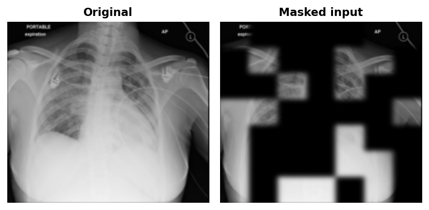
At epoch 50, blurry outlines were visible in the reconstructions.

By epoch 100, coarse lung field boundaries and rib cage structure were visible in the reconstructions.

By epoch 199, finer details like individual rib edges and lung vasculature emerged.
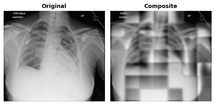
No matter what epoch, the patches will always be visible. This is a direct consequence of patchwise normalisation: the loss normalises each 32x32 patch to zero mean and unit variance independently before computing MSE. Adjacent predicted patches have slightly different overall exposure, and there is nothing in the loss to penalise that mismatch at the boundary, nor should it.
4.8 Cloud Training, Budgets, and Optimizers
Each method uses the optimizer from its original paper since the hyperparameters were derived under those assumptions.
1. MoCo v2: SGD, momentum 0.9, lr=4.5e-2 (linear-scaled from batch size: 0.03 × 384/256), weight decay 1e-4, 10-epoch warmup. SGD because the linear scaling rule in the original work assumes isotropic gradient steps; AdamW's per-parameter rescaling breaks that formula.
2. BarlowTwins: AdamW, lr=2.4e-3, weight decay 1e-4, 10-epoch warmup.
3. SparK: AdamW, lr=3.0e-4, weight decay 5e-2, 20-epoch warmup.
4. DINO: AdamW, lr=5.0e-4, weight decay 4e-2, 10-epoch warmup.
All runs use cosine annealing to 0 after warmup and mixed-precision training (torch.cuda.amp) throughout.


All pretraining ran on a Google Cloud L4: 22GB VRAM, 16 vCPU, 64GB RAM at ~$1.25/hr (g2-standard-16).
| Method | Backbone | Batch | Epochs | Failed runs | Final run | ~Total time | ~Cost |
|---|---|---|---|---|---|---|---|
| MoCo v2 | ResNet50 | 384 | 800 | 7 | 106h | ~149h | ~$187 |
| BarlowTwins | ResNet18 | 512 | 200 | 6 | 17h | ~18h | ~$22 |
| SparK | ResNet50 | 256 | 200 | 5 | 40h | ~40h | ~$50 |
| DINO | ResNet50 | 64 | ~5 (failed) | 10+ | — | ~30h | ~$38 |
| Total | ~237h | ~$297 |